ISNOBAL Adaptor Demo via an Experiment¶

The ISNOBAL model is widely used, but with little coherence between research groups. At least, this is what’s reflected in the lack of web-available tutorial-style documentation and lack of open source code for isnobal or for relevant IPW functions.

In this tutorial we follow the example experiment that’s written in examples/temperature_experiment.bash. Here we use all the tools of the isnobal_adaptor module of our adaptors project.

To get started, run the bash script listed above. If all is well, you can open the figure that gets saved as example_plot.png. For now it is pretty boring, since the demo is initially configured to only run with eleven input files.

To make a more interesting figure, you can make some modifications to the bash experiment script, but it will take much longer to run. In fact, you probably want to run it over night. On my MacBook Pro with 16GB of ram, an SSD hard drive, and an i7 processor it takes several hours to run the entire experiment. This can certainly be improved, but for our purposes at this time, this is good enough.

The Experiment: (How) does atmospheric temperature effect snow melt?¶

The iSNOBAL model takes a suite of inputs at each time step with 6 required input variables and possibly some precipitation variables if there was any precipitation in a given hour. One of the six required inputs is atmospheric temperature. Our experiment aims to answer the question, “What is the effect of increasing atmospheric temperature on snow melt?” Although to be complete scientifically we’d want to also consider secondary effects of increased temperature, like a higher percentage of rain to snow and changes in total precipitation, we only modify temperature and consider its effects.

Using observational data from the Kormos FTP site, we run the iSNOBAL model on the observed data, increase the atmospheric temperature by a given amount at every time step, run the iSNOBAL model for the observed input data and every modified set of input data, sum the total melting at each time step, saves the total melt by hour for each temperature scenario to a csv file, and plots the results. We do this by running the script, explained below.

Sub-scripts Used in the Experiment¶

In running the experiment, we use five separate Python scripts, shown in their entirety below. They can be run independently in an IPython shell (with run script.py) as well as from the command line.

A lot of the script is fancy stuff for downloading the files reliably and making sure our test case and full experiment both work.

Both the testing version and the full experiment download data from the “icewater” FTP site for the Kormos ISNOBAL paper

The test version downloads about 11 files and runs the experiment. For the test run, the resulting plot is pretty boring: there is only 11 hours worth of data and no snow to melt, so the graph is a flat line at zero kg/m^2.

To run the full experiment, search for comments that contain the string CHANGE FOR FULL. There you’ll find instructions on how to comment and uncomment the code that will result in either a test run or a full run.

Sub-script 1: Load a set of inputs; change `T_a` at every grid point and time step¶

#!/usr/local/bin/python
# assume observations are in obs_inputs/ and destination is inputs/

import os
import sys

from adaptors.src.isnobal_adaptor import IPW

# for simplicity, cl arg 1 is the source file, 2 is dest dir, and 3 is
# amount to change by
source_file = sys.argv[1]
dest_dir = sys.argv[2]
amount = float(sys.argv[3])

ipw = IPW(source_file)
ipw.dataFrame.T_a = ipw.dataFrame.T_a + amount
# required for proper writing. if new amounts exceed header max, trouble ensues..
ipw.recalculate_header()

output_file = dest_dir + os.path.basename(source_file)
ipw.write(output_file)

Sub-script 2: Generate CSV of total melt per hour from eight different “climate scenario” simulations¶

import os
import pandas as pd
import matplotlib.pyplot as plt

from adaptors.src.isnobal_adaptor import IPW
from collections import defaultdict

melt_sums = defaultdict(list)

for i, val in ["", "P0.5", "P1.0", "P1.5", "P2.0", "P2.5", "P3.0",
               "P3.5", "P4.0"]:

    dir_name = "outputs" + val

    files = ["/".join(dir_name, f) for f in os.listdir(dir_name)]

    melt_sums[val] = [IPW(f).dataFrame.melt.sum() for f in files]

index = pd.date_range('10/01/2010', periods=8758, freq='H')

df = pd.DataFrame(melt_sums, index=index)

df.to_csv("temperature_sensitivity_example.csv")

Sub-script 3: Resample output from the water melt example above¶

Read more about resampling with a pandas timeseries dataframe here, as well as this helpful stack overflow thread.

#!/usr/local/bin/python
import pandas as pd
import numpy as np

import matplotlib.pyplot as plt

from matplotlib import rcParams
rcParams.update({'figure.autolayout': True})

# nice looking plots are default with pandas
pd.options.display.mpl_style = "default"

# load data saved to csv from previous example
df = pd.read_csv("data/temperature_sensitivity_example.csv")
# have to re-assign because pandas doesn't parse it automatically. probably a
# way to tell it to read the index as a date_time.
df.index = pd.date_range('10/01/2010', periods=11, freq='H')

# TODO for full run, resample to 3-day sums
# df_3day = df.resample('3D', how=np.sum)

# set styles and plot
styles = ['-', '--', '-', '--', '-', '--', '-', '--', '-']

# TODO toggle commenting on next two lines when doing a full run
# ax = df_3day.plot(lw=3.5, style=styles)
ax = df.plot(lw=3.5, style=styles)

plt.title('Three-day sum of melt for observed/obs-plus temperatures',
          fontsize=12)
plt.xlabel('Date', fontsize=12)
plt.ylabel('Melt (kg/m^2)', fontsize=12)

# draw the legend in the upper-left corner
leg = plt.legend(loc=2, prop={'size': 7})

# set the linewidth of each legend object
for legobj in leg.legendHandles:
        legobj.set_linewidth(1.0)

ax.tick_params(axis='both', which='major', labelsize=8)
plt.savefig("example_plot.png", dpi=180, format='png')

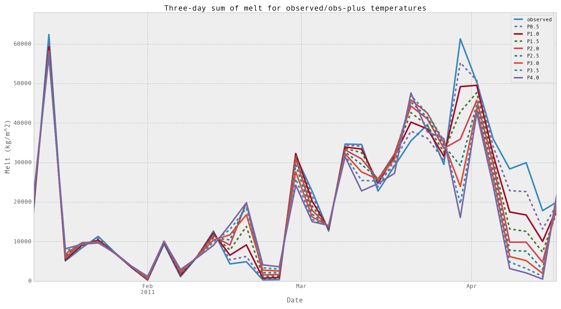
Resampled predictions for snowmelt over three day periods for various heating temps

We ran the ISNOBAL model for nine different temperatures, the observed temperatures from Kormos, et al., and then the observed heated by 0.5, 1.0, ..., 4.0 degrees Celsius. This is the output from the full experiment. Click to enlarge.

Other Sub-scripts¶

There are two other scripts, run_isnobal.py and recalc_input_headers.py. run_isnobal.py is a straight-forward wrapper of the adaptors.src.isnobal_adaptor.isnobal function, which in turn is a wrapper of the command-line isnobal command.

recalc_input_headers.py is required to transform the original data’s quantization to our quantization. Basically, in our implementation of calculating an IPW file’s header, we look at the maximum and minimum values present in the data, and then transform that to an integer with the original header-defined number of bytes.